从零开始学习机器学习：使用TensorFlow训练你的第一个神经网络：基本分类

在安装了TensorFlow 2.0之后，我们通过训练一个用于基本分类的神经网络，来熟悉TensorFlow的使用流程。这个神经网络可以用来分类服装图片，比如区分鞋子和T恤。

数据准备

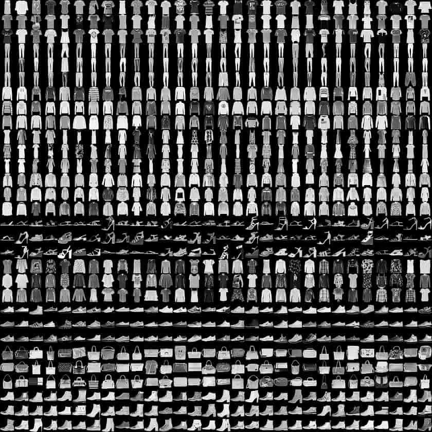
首先我们来看一下用于训练和测试模型的数据集Fashion MNIST。

Fashion MNIST是来自时尚服务平台Zalando的图片数据集，包含了60000张图片作为训练数据集，10000张图片作为测试数据集（更多关于Fashion-MNIST的信息可以查看：https://github.com/zalandoresearch/fashion-mnist）。

这个数据集如下图所示：

这个数据集并不需要我们自己去下载、处理，我们只需要通过Keras的接口进行调用即可。之前我们提到过，Keras是TensorFlow的一个高阶API。

from __future__ import absolute_import, division, print_function, unicode_literals

# TensorFlow and tf.keras
import tensorflow as tf
from tensorflow import keras

# Helper libraries
import numpy as np
import matplotlib.pyplot as plt

fashion_mnist = keras.datasets.fashion_mnist
(train_images, train_labels), (test_images, test_labels) = fashion_mnist.load_data()

train_images 和 train_labels 代表训练数据集和对应的标签，test_images 和 test_labels 代表测试数据集和对应的标签。标签是对应于图片的0—9的一组数字，代表的含义是：

class_names = ['T-shirt/top', 'Trouser', 'Pullover', 'Dress', 'Coat',
               'Sandal', 'Shirt', 'Sneaker', 'Bag', 'Ankle boot']

这样看似乎并不直观，我们可以通过matplotlib将加载的数据用图形的方式展示出来：

plt.figure()
plt.imshow(train_images[0])
plt.colorbar()
plt.grid(False)
plt.show()

在把数据导入模型前，我们需要做一些处理，保证里面的值的范围在0到1。因为数据集中的颜色是用0到255来表示，所以我们统一将数值除以255：

train_images = train_images / 255.0
test_images = test_images / 255.0

数据准备就绪，我们就可以进入正餐啦！

构建模型

1、Set up the layers（设置层）

一个神经网络最基本的单元就是"层"。这些层会从数据中抽取特征值。大部分的深度学习只需简单的将一些基本的层串联起来即可。

model = keras.Sequential([
    keras.layers.Flatten(input_shape=(28, 28)),
    keras.layers.Dense(128, activation='relu'),
    keras.layers.Dense(10, activation='softmax')
])

第一层tf.keras.layers.Flatten把二维数据（28 by 28）表示的图片信息，转化成一维（28 * 28 = 784）的数组。

第二第三层都是tf.keras.layers.Dense层，它们是全连接的。第二层有128个结点。第三层有10个结点，返回一个长度为10的数组，数组里包含的是概率，这些概率总和为1。

2、Compile the model（编译模型）

在模型可以训练前，还需要进行一些设置：

Loss function（损失函数）：损失函数是用来估量你模型的预测值f(x)与真实值Y的不一致程度

Optimizer（优化器）：机器学习中，有很多优化方法来试图寻找模型的最优解。比如神经网络中可以采取最基本的梯度下降法。

Metrics（指标）

model.compile(optimizer='adam',
              loss='sparse_categorical_crossentropy',
              metrics=['accuracy'])

开始训练

训练模型分为以下几步：

1）导入训练数据，这里就是图形数据和标签分类

2）模型学习关联图形和标签

3）使用模型对测试数据进行预测

使用model.fit开始训练：

model.fit(train_images, train_labels, epochs=10)

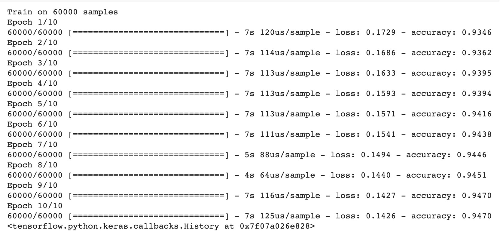
我们可以看到，精确度达到了94.7%

验证精度（Evaluate accuracy）

接下来看看这个模型在测试数据集上的表现：

test_loss, test_acc = model.evaluate(test_images, test_labels)
print('\nTest accuracy:', test_acc)

模型在测试数据集上的精确度为89.03%，尽管这是个不错的精确度，但还是远低于模型在训练数据集上的精确度。这种现象我们称之为过拟合（Overfitting）。

做预测（Make predictions）

模型训练之后，我们可以拿这个模型来给一些图片分类。

predictions = model.predict(test_images)

我们来看看第一张图片的预测结果：

predictions[0]

array([8.8770804e-07, 1.3376528e-07, 4.5999604e-09, 1.6275786e-10,
       7.0812092e-08, 9.2952169e-04, 2.1325867e-07, 1.1550661e-02,
       2.8679951e-08, 9.8751849e-01], dtype=float32)

之前我们说过，预测结果返回一个长度为10的数组，数组里包含的是概率，这些概率总和为1。那么，其中最大的值，就是模型预测最大概率的分类。

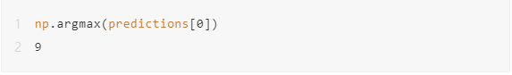
根据模型，第一张图片最有可能的分类是9。

我们再来看看人工标记的结果：

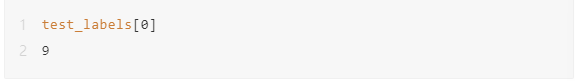
同样也是9。可见第一张图片，模型的分类与人工标记的结果一致！我们这就可以传入更多的图片，通过模型来预测其分类！

完整代码如下：

from __future__ import absolute_import, division, print_function, unicode_literals

# TensorFlow and tf.keras
import tensorflow as tf
from tensorflow import keras

# Helper libraries
import numpy as np
import matplotlib.pyplot as plt

print(tf.__version__)

fashion_mnist = keras.datasets.fashion_mnist
(train_images, train_labels), (test_images, test_labels) = fashion_mnist.load_data()

class_names = ['T-shirt/top', 'Trouser', 'Pullover', 'Dress', 'Coat',
               'Sandal', 'Shirt', 'Sneaker', 'Bag', 'Ankle boot']

train_images = train_images / 255.0
test_images = test_images / 255.0

model = keras.Sequential([
    keras.layers.Flatten(input_shape=(28, 28)),
    keras.layers.Dense(128, activation='relu'),
    keras.layers.Dense(10, activation='softmax')
])

model.compile(optimizer='adam',
              loss='sparse_categorical_crossentropy',
              metrics=['accuracy'])

model.fit(train_images, train_labels, epochs=10)

test_loss, test_acc = model.evaluate(test_images, test_labels)
print('\nTest accuracy:', test_acc)

predictions = model.predict(test_images)
print(predictions[0])
print(np.argmax(predictions[0]))
print(test_labels[0])